davidegazze.github.io
A gentle introduction to Data Synthetic Data Quality Metrics
In my previous post [1], I introduced the SDV package, a powerful library to generate synthetic data from an original dataset. In [2], I showed some advanced features like Constraints and Anonymization. This article will introduce some data quality metrics to evaluate the synthetic data. Of course, the introduced metric can be important in many fields, either in Data Science or Data Engineering Applications. For this reason, I go deeper into this field. This post is the result of my study. To evaluate the Data Quality, DataCebo helps us with the project SDMetrics [3]. SDMetrics is a model-agnostic package that can score the data quality of synthetic data concerning the original one. Moreover, you can use this package to compare two datasets not generated by SDV. This could open new opportunities in Data Quality in general. In this case, the library can be used to evaluate the data quality of one dataset relative to another. This post will introduce the SDMetrics library to analyze metrics in data quality. So we can have twofold feedback: learning a new library and having a blueprint for evaluating data quality in a generic project.
Installation
As usual, you have to install the package:
pip install sdmetrics
To begin, you will need the following:
- The original data as pandasDataFrame
- The new data as pandas DataFrame
- Metadata of the data
Metrics Supported
From [4], we can see the kind of metrics that the package supports. The list is very long. Moreover, you can use some ad-hoc metrics. We can divide the metrics into 4 classes:
- Single Column to compare single columns of data;
- Column Pairs to compare pairs of columns;
- Single Table to a table of data;
- Multi Tables to compare multiple tables of data.
Single Columns Metrics
CategoryCoverage
CategoryCoverage [6] metric can measure whether a column covers all the possible categories. This metric works with Categorical and Boolean data. The output is a score:
- (best) 1.0: The new column contains all the categories present in the original column
- (worst) 0.0: The new column does not contain the categories present in the original column
The score is calculated with the formula:
$$
score=\frac{cs}{cr}
$$
Where cr is the number of categories in the original column, and cs is the categories’ number in the new one.
A simple way to calculate this metric is the following:
from sdmetrics.single_column import CategoryCoverage

CategoryCoverage.compute(
    real_data=original_table['column_name'],
    synthetic_data=new_table['column_name']
)
RangeCoverage
This metric [7] measures whether a new column covers the full range of values from an original column.
This metric works well with Numerical and Datetime values.
The score goes from 1 (the best) to 0 (the worst) if the new column does not overlap at all with the range of values in the original one.
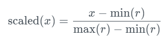
The formula is:
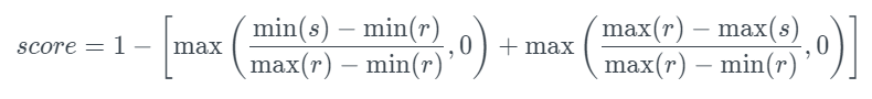
This metric calculates how closely the minimum and maximum values of a new column (s) match the minimum and maximum values of an original column (r). A score of 0 is given if the new dataset has poor range coverage, while a score of 1 is assigned if the new dataset covers the entire range, even exceeding the boundaries of the original data.
To use these metrics, you can use the following:
from sdmetrics.single_column import RangeCoverage

RangeCoverage.compute(
    real_data=original_table['column_name'],
    synthetic_data=new_table['column_name']
)
BoundaryAdherence
This metric [8] assesses whether a new column adheres to the minimum and maximum values of the original column. It provides the percentage of new rows that fall within the boundaries of the original data. Data Compatibility:
- Numerical: This metric is designed for numerical data.
- Datetime: This metric converts datetime values into numerical values.
This metric disregards missing values.
The score goes from 0 to 1:
- (best) 1.0: All values in the new column adhere to the minimum and maximum boundaries of the original data.
- (worst) 0.0: No value in the new column falls within the range defined by the minimum and maximum values of the original data.
An example of how to use this metric is:
from sdmetrics.single_column import BoundaryAdherence

BoundaryAdherence.compute(
    real_data=original_table['column_name'],
    synthetic_data=new_table['column_name']
)
KSComplement The Kolmogorov-Smirnov (KS) metric [9].
This metric compares the distribution of the original and new columns. It is designed for continuous numerical data and converts date values into numerical values. The KSComplement uses the Kolmogorov-Smirnov statistic. It is the maximum difference between the two cumulative distribution functions (CDFs). The KS statistic can determine the compatibility of original and new data. Score: *(best) 1.0: The original data is identical to the new data (worst).
- 0.0: The original and new data are as dissimilar as can be.
The Kolmogorov-Smirnov statistic [1] is used by the KSComplement. This statistic is computed by converting a numerical distribution into its cumulative distribution function (CDF) [2]. As shown below, the KS statistic is the maximum difference between the two CDFs.
The distance is represented by a number between 0 and 1. SDMetrics inverts the statistic: The KSComplement function returns 1-(KS statistic), so a higher score indicates higher quality. To compute this metric:
from sdmetrics.single_column import KSComplement

KSComplement.compute(
    real_data=original_table['column_name'],
    synthetic_data=new_table['column_name']
)
TVComplement
This metric [10] computes the similarity of an original column to a new column in terms of the column’s marginal distribution or 1D histogram for Categorical and Boolean values.
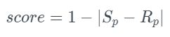
The Total Variation Distance (TVD) between the original and new columns is calculated using this test. To accomplish this, it first computes and expresses the frequency of each category value as a probability. The TVD statistic compares probability differences, as shown in the formula below [1]:
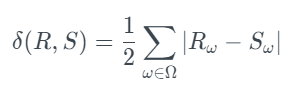
In this case, describes all the possible categories in a column. Meanwhile, R and S are the original and new frequency columns. The TVComplement returns 1-TVD, so a higher score indicates better quality. The score is:
To use this metric:
from sdmetrics.single_column import TVComplement

TVComplement.compute(
    real_data=original_table['column_name'],
    synthetic_data=new_table['column_name']
)
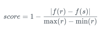
StatisticSimilarity
This metric [11] compares a summary statistic to determine the similarity between an original and a new column. The following summary statistics are supported: mean, median, and standard deviation. Compatibility of Data This metric is intended for continuous, numerical data. Moreover, the datetime values are converted to numbers. Missing values are ignored by this metric. A score goes from 0.0 (the minimum) to 1.0 (the best score). The given statistical function, f, is computed for the original data and new columns, r, and s, in this test. The score is then normalized by scaling and taking its complement. This yields a score in the [0, 1] range*, with a high value indicating high similarity.
To use this metric:
from sdmetrics.single_column import StatisticSimilarity

StatisticSimilarity.compute(
    real_data=original_table['column_name'],
    synthetic_data=new_table['column_name'],
    statistic='mean'
)
Where statistic: A string describing the name of the statistical function:
- (default) ‘mean’: The arithmetic mean
- ‘median’: The median value
- ‘std’: The standard deviation
MissingValueSimilarity
This metric [12]
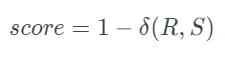
It compares whether the new data for a given column has the same proportion of missing values as the original data. The metrics work with all data types and can handle missing values. The best score is 1.0, and the worst is 0.0. This test computes the proportion of missing values, p, in the original and new data, R and S. It normalizes them and returns a similarity score in the range [0, 1], with 1 representing the highest similarity.
It should be noted that the term on the right corresponds to the Total Variation Distance [1] of the missing/non-missing values between the original and new data.
An example of how to use this metric is:
from sdmetrics.single_column import MissingValueSimilarity

MissingValueSimilarity.compute(
    real_data=original_table['column_name'],
    synthetic_data=new_table['column_name']
)
Column Pairs Metrics
These metrics refer to pairs of columns.
ContingencySimilarity
This metric [13] compares 2D distributions by computing the similarity of two categorical columns in the original and new datasets. This metric applies to Categorical and Boolean data types. Both columns must be compatible to use this metric. If both columns have missing values, the metric will treat them as a separate, single category.
The score has the following values:
- (best) 1.0: The contingency table is identical between the original and new data.
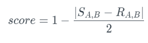
- (worst) 0.0: The contingency table is as unique as they come. The test computes a normalized contingency table for the original and new data. The formula below summarizes the process.
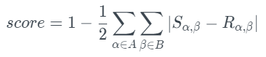
The image above describes all possible categories in column A and all possible categories in column B in the formula. Meanwhile, R and S denote the original and new frequencies.
To run this metric manually, go to the column_pairs module and use the compute method:
from sdmetrics.column_pairs import ContingencySimilarity

ContingencySimilarity.compute(
    real_data=original_table[['column_1', 'column_2']],
    synthetic_data=new_table[['column_1', 'column_2']]
)
CorrelationSimilarity
This metric [14] computes the similarity between original and new data and measures the correlation between two numerical columns, i.e., compares the trends of two-dimensional distributions. This metric can accept Pearson’s and Spearman’s rank coefficients to measure the correlation. This metric accepts Numeric and DateTime values.
The score is based on the following values:
- (best) 1.0: The pairwise correlations of original and new data are identical;
- (worst) 0.0: The pairwise correlations are as dissimilar.
This test computes a correlation coefficient on original and new data, R and S, for a pair of columns. This results in two distinct correlation values. The test normalizes and returns a similarity score.
It should be noted that the correlation coefficient can be calculated in different ways. Both the Pearson correlation coefficient and Spearman’s rank correlation coefficient are supported. Both have a range of -1 to +1. In Data Science, the Pearson and Spearman rank correlation coefficients are frequently used. The Pearson coefficient determines whether two columns are linearly related, whereas the Spearman coefficient determines whether they are monotonically related. Both coefficients are between -1 and +1. The table below provides a rough interpretation. To run this metric manually, go to the column_pairs module and use the compute method:
from sdmetrics.column_pairs import CorrelationSimilarity

CorrelationSimilarity.compute(
    real_data=original_table[['column_1', 'column_2']],
    synthetic_data=new_table[['column_1', 'column_2']],
    coefficient='Pearson'
)
Single Table Metrics
These metrics refer to a table.
NewRowSynthesis
This metric [15] determines whether each row in the new data is unique or identical to an original row in the original data. This metric works with all data types, including categorical, Boolean, numeric, and datetime. This metric looks for matches in missing values as well. It disregards any additional columns in your data. The score has the following value ranges:
- (best) 1.0: All the rows in the synthetic data are unique. There are no matches with real-world data.
- (worst) 0.0: All of the rows in the synthetic data are duplicates of real-world rows.
This metric looks for rows that match the original and the new datasets. The exact matching criteria are determined by the type of data.
The match is considered when the synthetic value is within a %. The % is a parameter that is, by default, set to 0.01 (1%). For a match to be considered, both original and new values must be missing. The complement is the score, so 1 is a good score (every row is unique), and 0 is the worst (every row has a match).
An example of how to use this metric is:
from sdmetrics.single_table import NewRowSynthesis

NewRowSynthesis.compute(
    real_data=original_table,
    synthetic_data=new_table,
    metadata=single_table_metadata_dict,
    numerical_match_tolerance=0.01,
    synthetic_sample_size=10_000
)
CategoricalCAP
The CategoricalCAP [16] assesses the risk of sensitive information being disclosed via an inference attack. We assume that some values in the real data are known to the public. An attacker combines this with synthetic data to make educated guesses about other sensitive real-world values. Using an algorithm called Correct Attribution Probability (CAP), this metric describes how difficult it is for an attacker to correctly guess sensitive information.
This metric is compatible with Categorical and Boolean values.
As usual, the score goes from 0.0 to 1.0. A value of 1.0 means that an attacker is not able to guess the sensitive values.
More information is available in [18].
An example of how to use this metric is:
from sdmetrics.single_table import CategoricalCAP

score = CategoricalCAP.compute(
    real_data=original_table,
    synthetic_data=new_table,
    key_fields=['age_bracket', 'gender'],
    sensitive_fields=['political_affiliation']
)
The key_fields represents the list of column names to attack.
The sensitive_fields is a list of the column names that the attacker would guess.
Multi Tables Metrics
These metrics are used in more tables.
CardinalityShapeSimilarity
If you have multiple tables that are connected, the CardinalityShapeSimilarity metric
[17]
determines whether the cardinality of the parent table is the same in the real and synthetic datasets.
The number of child rows for each parent is defined as the cardinality.
The score goes from 0.0 to 1.0:
- (best) 1.0: The cardinality values are the same
- (worst) 0.0: The cardinality values are different
An example of the use of this metric is the following:
from sdmetrics.multi_table import CardinalityShapeSimilarity

CardinalityShapeSimilarity.compute_breakdown(
    real_data={
      'user': real_user_table,
      'sessions': real_sessions_table,
      'transactions': real_transactions_table
    },
    synthetic_data={
      'users': synthetic_user_table,
      'sessions': real_sessions_table,
      'transactions': real_transactions_table
    },
    metadata=multi_table_metadata_dict
)
Metrics in beta
From the [5], there are many beta metrics.
Why are there in beta? The SDMetrics library is to provide high-quality, mathematically sound, and vetted metrics. However, the synthetic data field is a relatively new area with active research. So these metrics are for anyone interested in experimenting with them.
Summary
Thank you for reading my post. I hope that it has been interesting for you as it has been for me. The Data Quality field is exciting, and it is precious to improve this skill before putting production something wrong.
References
- SDV: Generate Synthetic Data using GAN and Python
- Adding Constraints and Anonymization to SDV Models
- SDMetrics
- Metrics Glossary
- Metrics in Beta
- CategoryCoverage
- RangeCoverage
- BoundaryAdherence
- KSComplement
- TVComplement
- StatisticSimilarity
- MissingValueSimilarity
- ContingencySimilarity
- CorrelationSimilarity
- NewRowSynthesis
- CategoricalCAP
- CardinalityShapeSimilarity
- The CAP Algorithm